1. Problem Statement:
- 1.1. Introduction:
- 1.2. Problem:
2. Motivation:
3. Dataset:
- 3.1. Data Resource:
- 3.2. Data Overview:
4. Approach:
- 4.1. How probability was calculated?
5. Analysis of Dataset:
- 5.1. Visualization
6. Feature Engineering
7. Model Building
8. Training, Validation and Test Metrics.
9. Sources And References.
10. Conclusion

Problem Statement:

Introduction:

Discussing things you care about can be difficult. The threat of abuse and harrasment online means that many people stop experssing themselves and give up on seeking different opinions. Platforms struggle to efficiently facilitate conversations, leading many communities to limit or completely shut down user comments.

Problem:

Building a multi-headed model that’s capable of detecting different types of toxicity like threats, obscenity, insult and identity-based hate.

Motivation:

So far we have a range of publicly available models served through the Perspective API, including toxicity. But the current models still make errors, and they don’t allow users to select which type of toxicity they’re interested in finding. (e.g. some platforms may be fine with profanity, but not with other types of toxic content)

Dataset:

Data Resource:

The dataset used was Wikipedia corpus dataset which was rated by human raters for toxicity. The corpus contains comments from discussions relating to use pages and articles dating from 2004-2015. The dataset was hosted on Kaggle.

Data Overview:

The comments were manually classified into following categories

toxic
severe_toxic
obscene
threat
insult
identity_hate

The Dataset had 150k comments which were classified into one or more above categories. The problem was to predict the probabilities of 10k comments being classified into multiple categories.

Approach:

How probability was calculated?

Though there many multi class classifiers, we didn’t find a suitable multi label classifier which was able to give probability with which target belongs to a label.

So, we used scikit-learn OneVsRestClassifier with various estimators, with the help of predict_proba, we predicted the probability with which a comment belongs to a particular label.

Analysis of Dataset:

Visualization

Count of number of comments in each class.

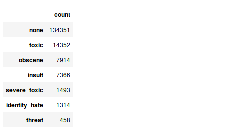
The three major labels are:

toxic
obscene
insult

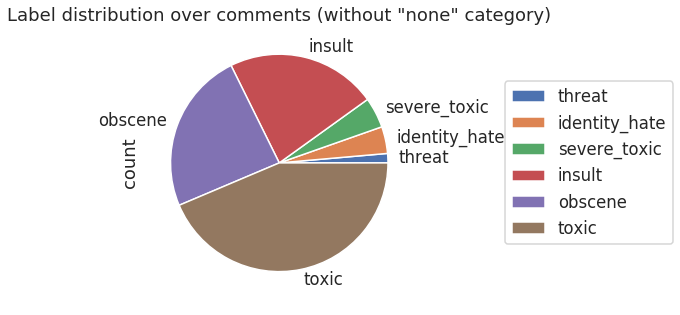
Pie chart of Label Distribution over comments(without “none” category).

Count for each label combination.

Now, let’s take a look at number of comment for each label combination.This helps us in finding correlation between categories. \newline

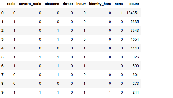
Following can be inferred from above table:

The table shows that number of comments with only none label are high.
toxic which is the lable high after none is present in all top 6 combinations.
Among the top combinations, obscene and insult comes 4 times in 6.
As the combinations increase (i.e, a comment belonging to more categories) the count drops very fast.

Correlation matrix.

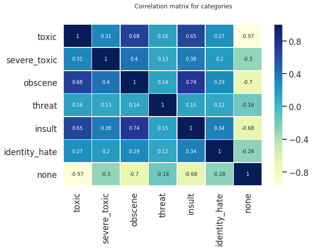
Following can be inferred from above matrix:

Toxic is highly correlated with obscene and insult
Insult and obscene have highest correlation factor of (0.74)

Interesting things to be observed:

Though a severe toxic comment is also a Toxic comment, the correlation between them is only 0.31.

Digging more into correlations using Venn Diagrams.

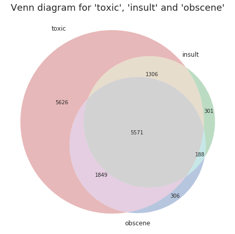
This venn diagram shows the interpretations inferred from the correlation matrix above.

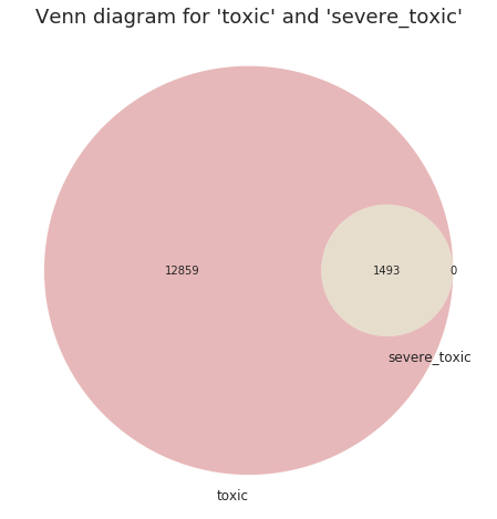
This venn diagram shows that if a comment is severe toxic it indeed is also a toxic comment.
The low correlation factor is explained by the fact that severe toxic represents a small percentage to toxic. This is similar to Simpson’s Paradox.

Word analysis for each cateogires.

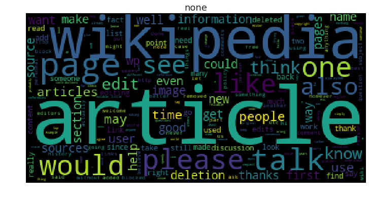
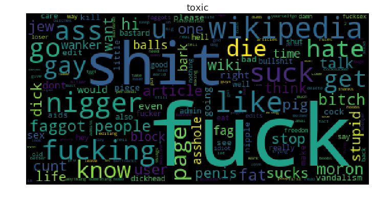
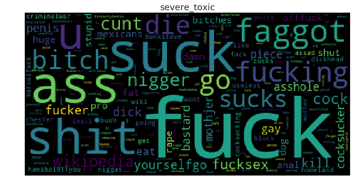
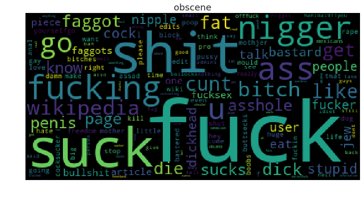
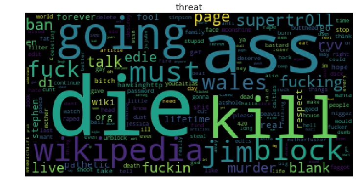
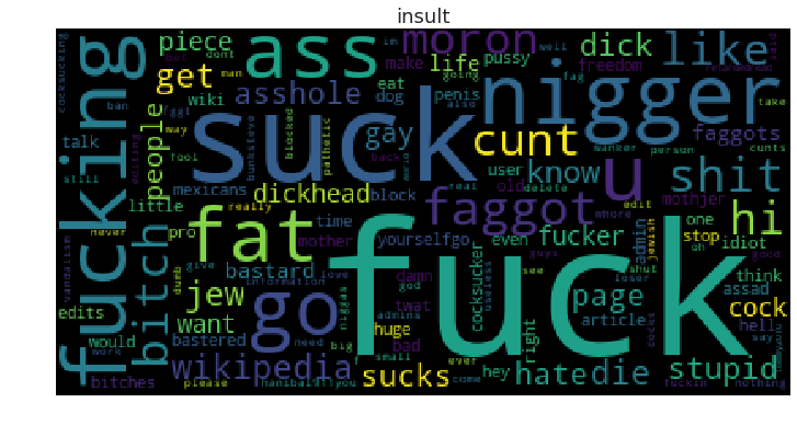
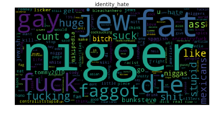
The vocabulary used in all categories is quite similar.

Feature Engineering

Cleaning the comments

Since, the comments in the dataset were collected from the internet they may contain ‘HTML’ elements in them. So, we removed the HTML from the test by using BeautifulSoup.
```
review_text = BeautifulSoup(raw_review).get_text()
```
We then converted each comment into lower case and then splitted it into individual words.
```
words = review_text.lower().split()
```
There were some words in the dataset which had length > 100, since there are no words in the english language whose length > 100, we wrote a function to remove such words.
```
def remove_big_words(words):
l = []
for word in words:
    if len(word) <= 100:
        l.append(word)
return l
```
First, we tried building the features removing stop words and then trained some models thinking that it may help the model in learning the semantics of toxicity, but we found out that the model learns better if there are stop words in the comment.

Possible reason is, generally a hate/toxic comment is used towards a person, seeing the data we found out that those persons are generally referred by pronouns, which are nothing but stop words.

Stemmers and Lemmatizers

Definitions:
- Stemming usually refers to a crude heuristic process that chops off the ends of words in the hope of achieving this goal correctly most of the time, and often includes removal of derivational affixes.
- Lemmatization usually refers to doing things properly with the use of a vocabulary and morphological analysis of words, normally aiming to remove inflectional endings only and to return the base or dictionary form of a word, which is known as the lemma.
  
  (Definitions source: stemming and Lemmatization)
Reasons to use:
- We used both snowball stemmer, porter stemmer and wordnet lemmatizer.
- For gramatical reasons, documents are going to use different forms of a word, such as organizes, organize and organizing. But they all represent the same semantics. So, using stemmer/Lemmatizer for those three words gives a single word, which helps algorithm learn better.
Results:
- On public Dataset: (Decreasing order of accuracy)
  
  Snowball Stemmer > WordNet Lemmatizer > Porter Stemmer
- On private Dataset: (Decreasing order of accuracy)
  
  WordNet Lemmatizer > Snowball Stemmer > Porter Stemmer

Vectorization

Python’s scikit-learn deals with numeric data only. To conver the text data into numerical form, tf-idf vectorizer is used. TF-IDF vectorizer converts a collection of raw documents to a matrix of Tf-idf features.

We fit the predictor variable on the dataset with tf-idf vectorizer, in two different ways. First, by setting the parameter analyzer as ‘word’(select words) and the second by setting it to ‘char’(select characters). Using ‘char’ was important because the data had many ‘foreign languages’ and they were difficult to deal with by considering only the ‘word’ analyzer.

We set the paramater n-gram range (an n-gram is a continguous sequence of n-items from a given sample of text or speech). After trying various values, we set the ngram as (1, 1) for ‘word’ analyzer and (1, 4) for ‘char’ analyzer. We also set the max_features as 30000 for both word and char analyzer after many trails.

We then combined the word and character features and transformed the dataset into two sparse matrixes for train and test sets, respectively using tf-idf vectorizer.

We tried adding features to the dataset that are computed from the data itself. Those features are:

Length of comments
Number of exclamation marks - Data showed severe toxic comments with multiple exclamation marks.
Number of question marks
Number of punctuation symbols - Assumption is that angry people might not use punctuation symbols.
Number of symbols - there are some comments with words like f**k, $#*t etc.
Number of words
Number of unique words - Data showed that angry comments are sometimes repeated many times.
Proportion of unique words

Correlation between above features and labels:

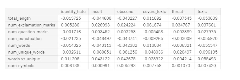
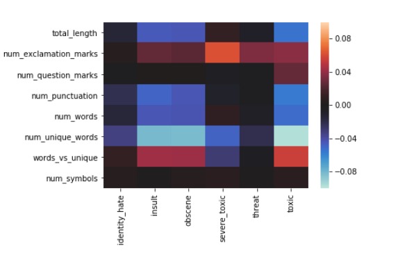
Conclusion from above correlation matrix:

All the above features had correlation of < 0.06 with all labels. So, we decided that adding these features doesn’t give benefit the model.

Model Building

Our basic pipeline consisted of count vectorizer or a tf-idf vectorizer and a classifier. We used OneVsRest Classifier model. We trained the model with Logistic Regression (LR), Random Forest(RF) and Gradient Boosting(GB) classifiers. Among them LR gave good probabilities with default parameters.

So, we then improved the LR model by changing its parameters.

Training, Validation and Test Metrics.

Training and Validation split:

To know whether was generalizable or not, we divided the into train and validation sets in 80:20 ratio. We then trained various models on the training data, then we ran the models on validation data and we checked whether the model is generalizable or not.

Also, we trained different models on training data and tested those on validation data, then we arrived at our best model.

Test Metric:

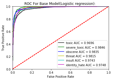
We used Receiver Operating Characteristic(ROC) along with Area under the curve(AUC) as test metric.

Results for various models.

Base model:

We created a model without any preprocessing or parameter tuning, we used this model as our model, and measured our progress using this model.

For this we used Logistic Regression as Classifier.

Cross Validation Results.

Category CV Score

Toxic 0.9501

Severe\_toxic 0.9795

Obscene 0.9709

Threat 0.9733

Insult 0.9608

Identity\_hate 0.9548

Average CV 0.9649
ROC-AUC Curve.

Category	CV Score
Toxic	0.9501
Severe\_toxic	0.9795
Obscene	0.9709
Threat	0.9733
Insult	0.9608
Identity\_hate	0.9548
Average CV	0.9649

Random Forest:

Next, we created our model using Random Forest. We used n_estimators = 10 and random_state = 1 as parameters.

We observed the following results

Cross Validation Results.

Category CV Score

Toxic 0.8984

Severe\_toxic 0.8479

Obscene 0.9491

Threat 0.6816

Insult 0.9183

Identity\_hate 0.7782

Average CV 0.7782
ROC-AUC Curve.

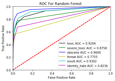
From the Cross Validation results table and ROC-AUC Curve, its clear that Random Forest performs poorly compared to our base model itself, So we proceeded to tune parameters for Logistic Regression for better accuracy.

Category	CV Score
Toxic	0.8984
Severe\_toxic	0.8479
Obscene	0.9491
Threat	0.6816
Insult	0.9183
Identity\_hate	0.7782
Average CV	0.7782

Logistic Regression:

(I)

We created one model using C = 4 as parameter. The following results were observed.

Cross Validation Results:

Category CV Score

Toxic 0.9690

Severe\_toxic 0.9850

Obscene 0.9825

Threat 0.9856

Insult 0.9750

Identity\_hate 0.9774

Average CV 0.9791

Category	CV Score
Toxic	0.9690
Severe\_toxic	0.9850
Obscene	0.9825
Threat	0.9856
Insult	0.9750
Identity\_hate	0.9774
Average CV	0.9791

ROC-AUC Curve.

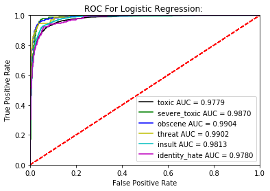
(II)

We created another Logistic Regression by selecting the best parameters by crossvalidating the following parameters.

C	fit\_intercept	penalty	class\_weight
1.05	True	'l2'	None
0.2	True	'l2'	'balanced'
0.6	True	'l2'	'balanced'
0.25	True	'l2'	'balanced'
0.45	True	'l2'	'balanced'
0.25	True	'l2'	'balanced'

Cross Validation Results:

Category CV Score

Toxic 0.9675

Severe\_toxic 0.9864

Obscene 0.9827

Threat 0.9847

Insult 0.9761

Identity\_hate 0.9764

Average CV 0.9790
ROC-AUC Curve.

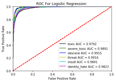
Though, (I) gave better score compared to (II) on validation set, with difference in order of 0.0001. when run on the acutal data (II) was found to better than (I)

Category	CV Score
Toxic	0.9675
Severe\_toxic	0.9864
Obscene	0.9827
Threat	0.9847
Insult	0.9761
Identity\_hate	0.9764
Average CV	0.9790

Sources And References.

Conclusion

After checking the kaggle discussion board of the actual competition, standard Machine Learning approaches yield a maximum score of 0.9792, irrespective of any aprroach. In order to get a large margin over this score one has to employ Deep Learning(DL) techniques.

Toxic Comments Classification

Table of Contents